class10

The PDB database

The Protein Data Bank (PDB) is the main repository of biomolecular structure data . Let’s see what is in it:

stats <- read.csv("pdb_stats.csv", row.names = 1)
stats

                         X.ray    EM   NMR Integrative Multiple.methods Neutron
Protein (only)          178795 21825 12773         343              226      84
Protein/Oligosaccharide  10363  3564    34           8               11       1
Protein/NA                9106  6335   287          24                7       0
Nucleic acid (only)       3132   221  1566           3               15       3
Other                      175    25    33           4                0       0
Oligosaccharide (only)      11     0     6           0                1       0
                        Other  Total
Protein (only)             32 214078
Protein/Oligosaccharide     0  13981
Protein/NA                  0  15759
Nucleic acid (only)         1   4941
Other                       0    237
Oligosaccharide (only)      4     22

Q1: What percentage of structures in the PDB are solved by X-Ray and Electron Microscopy.

n.sums <- colSums(stats)
n <- n.sums/n.sums["Total"]
round(n, digits=2)

           X.ray               EM              NMR      Integrative 
            0.81             0.13             0.06             0.00 
Multiple.methods          Neutron            Other            Total 
            0.00             0.00             0.00             1.00 

81% for X-Ray and 13% for Electron Microscopy

What is the total number of entries in the PDB?

n.sums["Total"]

 Total 
249018 

Q2: What proportion of structures in the PDB are protein?

Q3: Type HIV in the PDB website search box on the home page and determine how many HIV-1 protease structures are in the current PDB?

Using Molstar

We can use the main Molstar viewer online:

First view of HIV-Pr dimer with bound inhibitor

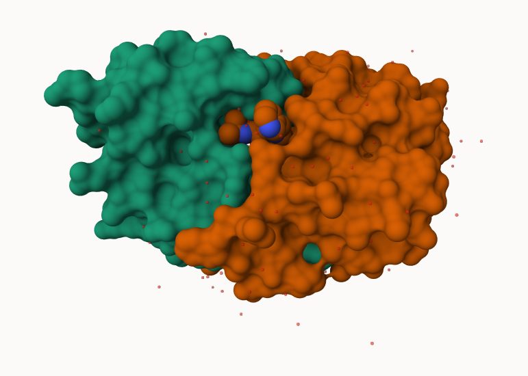
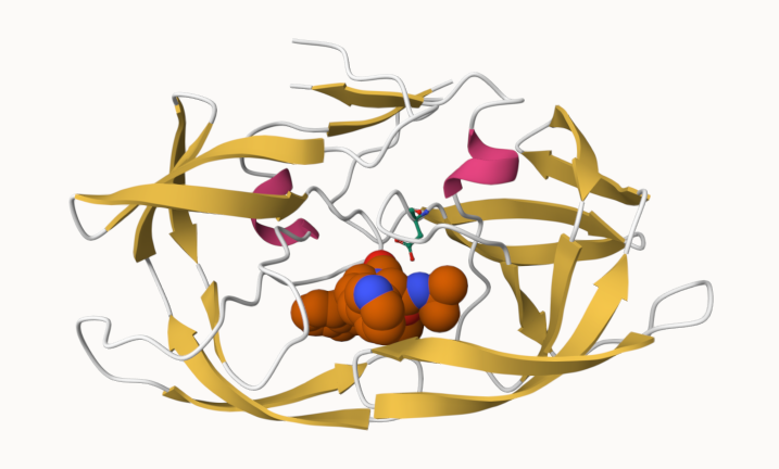
Q. Generate and insert an image of the HIV-Pr cartoon colored by secondary structure, showing the inhibitor (ligand) in spacefill.

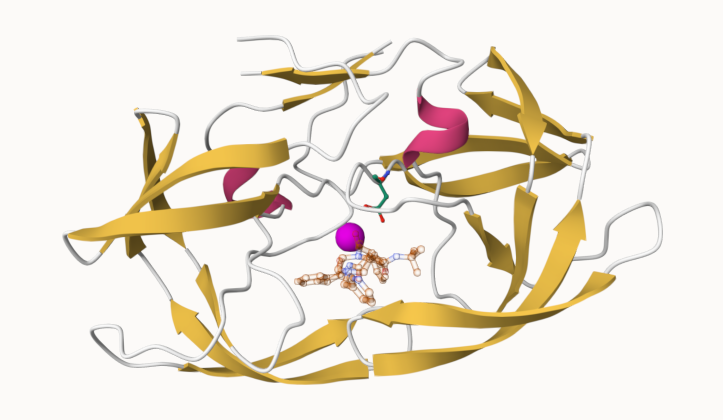
Q. One fimal image showing catalytic APS 25 and the all-important active site water molecule.

The bio3D package for structural bioinformatics

library(bio3d)

hiv <- read.pdb("1hsg")

  Note: Accessing on-line PDB file

hiv

 Call:  read.pdb(file = "1hsg")

   Total Models#: 1
     Total Atoms#: 1686,  XYZs#: 5058  Chains#: 2  (values: A B)

     Protein Atoms#: 1514  (residues/Calpha atoms#: 198)
     Nucleic acid Atoms#: 0  (residues/phosphate atoms#: 0)

     Non-protein/nucleic Atoms#: 172  (residues: 128)
     Non-protein/nucleic resid values: [ HOH (127), MK1 (1) ]

   Protein sequence:
      PQITLWQRPLVTIKIGGQLKEALLDTGADDTVLEEMSLPGRWKPKMIGGIGGFIKVRQYD
      QILIEICGHKAIGTVLVGPTPVNIIGRNLLTQIGCTLNFPQITLWQRPLVTIKIGGQLKE
      ALLDTGADDTVLEEMSLPGRWKPKMIGGIGGFIKVRQYDQILIEICGHKAIGTVLVGPTP
      VNIIGRNLLTQIGCTLNF

+ attr: atom, xyz, seqres, helix, sheet,
        calpha, remark, call

head( hiv$atom )

  type eleno elety  alt resid chain resno insert      x      y     z o     b
1 ATOM     1     N <NA>   PRO     A     1   <NA> 29.361 39.686 5.862 1 38.10
2 ATOM     2    CA <NA>   PRO     A     1   <NA> 30.307 38.663 5.319 1 40.62
3 ATOM     3     C <NA>   PRO     A     1   <NA> 29.760 38.071 4.022 1 42.64
4 ATOM     4     O <NA>   PRO     A     1   <NA> 28.600 38.302 3.676 1 43.40
5 ATOM     5    CB <NA>   PRO     A     1   <NA> 30.508 37.541 6.342 1 37.87
6 ATOM     6    CG <NA>   PRO     A     1   <NA> 29.296 37.591 7.162 1 38.40
  segid elesy charge
1  <NA>     N   <NA>
2  <NA>     C   <NA>
3  <NA>     C   <NA>
4  <NA>     O   <NA>
5  <NA>     C   <NA>
6  <NA>     C   <NA>

pdbseq(hiv)

  1   2   3   4   5   6   7   8   9  10  11  12  13  14  15  16  17  18  19  20 
"P" "Q" "I" "T" "L" "W" "Q" "R" "P" "L" "V" "T" "I" "K" "I" "G" "G" "Q" "L" "K" 
 21  22  23  24  25  26  27  28  29  30  31  32  33  34  35  36  37  38  39  40 
"E" "A" "L" "L" "D" "T" "G" "A" "D" "D" "T" "V" "L" "E" "E" "M" "S" "L" "P" "G" 
 41  42  43  44  45  46  47  48  49  50  51  52  53  54  55  56  57  58  59  60 
"R" "W" "K" "P" "K" "M" "I" "G" "G" "I" "G" "G" "F" "I" "K" "V" "R" "Q" "Y" "D" 
 61  62  63  64  65  66  67  68  69  70  71  72  73  74  75  76  77  78  79  80 
"Q" "I" "L" "I" "E" "I" "C" "G" "H" "K" "A" "I" "G" "T" "V" "L" "V" "G" "P" "T" 
 81  82  83  84  85  86  87  88  89  90  91  92  93  94  95  96  97  98  99   1 
"P" "V" "N" "I" "I" "G" "R" "N" "L" "L" "T" "Q" "I" "G" "C" "T" "L" "N" "F" "P" 
  2   3   4   5   6   7   8   9  10  11  12  13  14  15  16  17  18  19  20  21 
"Q" "I" "T" "L" "W" "Q" "R" "P" "L" "V" "T" "I" "K" "I" "G" "G" "Q" "L" "K" "E" 
 22  23  24  25  26  27  28  29  30  31  32  33  34  35  36  37  38  39  40  41 
"A" "L" "L" "D" "T" "G" "A" "D" "D" "T" "V" "L" "E" "E" "M" "S" "L" "P" "G" "R" 
 42  43  44  45  46  47  48  49  50  51  52  53  54  55  56  57  58  59  60  61 
"W" "K" "P" "K" "M" "I" "G" "G" "I" "G" "G" "F" "I" "K" "V" "R" "Q" "Y" "D" "Q" 
 62  63  64  65  66  67  68  69  70  71  72  73  74  75  76  77  78  79  80  81 
"I" "L" "I" "E" "I" "C" "G" "H" "K" "A" "I" "G" "T" "V" "L" "V" "G" "P" "T" "P" 
 82  83  84  85  86  87  88  89  90  91  92  93  94  95  96  97  98  99 
"V" "N" "I" "I" "G" "R" "N" "L" "L" "T" "Q" "I" "G" "C" "T" "L" "N" "F" 

Let’s try out the new bio3dview package that is not yet on CRAN. We can use the remotes package to install any R package from GitHub.

Quick viewing of PDBs

library(bio3dview)

sele <- atom.select(hiv, resno=25)
view.pdb(hiv, backgroundColor = "pink",
         highlight = sele,
        highlight.style = "spacefill")

Prediction of Protein flexiblity

adk <- read.pdb("6s36")

  Note: Accessing on-line PDB file
   PDB has ALT records, taking A only, rm.alt=TRUE

m <- nma(adk)

 Building Hessian...        Done in 0.09 seconds.
 Diagonalizing Hessian...   Done in 0.73 seconds.

plot(m)

Write out our results as a wee trajectory movie:

mktrj(m, file="results.pdb")

view.nma(m)